bugarachA coordinated-event detector, trained on data that is hard to label reliably.

Five detector lanes above a 30-ROI raster and five analysis traces.
Each lane marks where that detector called a coordinated event;
the shaded block is a dense-but-random stretch containing none. — **Thirty minutes of simulated recording, and what five detectors made of it.** One lane per detector, each bar a call it made; then the raster they were all reading, one row per ROI; then what each detector computes. Each lane carries its detector's own name; two of the five are named for what they measure rather than for the tool — rate+context is RateDetect, and binned SCE is SCE. In the lanes, ✗ marks a false alarm and ◯ one that a reader should not count as a separate miss-fire — a second call on an event another detection had already claimed, or one too close to this detector's own hit for the picture to separate. The bars are the windows the detectors called: most run under two seconds, which is about a pixel at this width, so they are hairlines; SCE bins at ten seconds and its bars are wider because they are. The top lane is the ground truth, and every mark in it points down at the raster it is about: a green ▼ is an event some detector recovered, a red ▼ one they all missed. The shaded block fires at a higher rate but contains **no planted events**, so every bar inside it is a false alarm by construction — you can see which detectors take the bait. Open the interactive version →

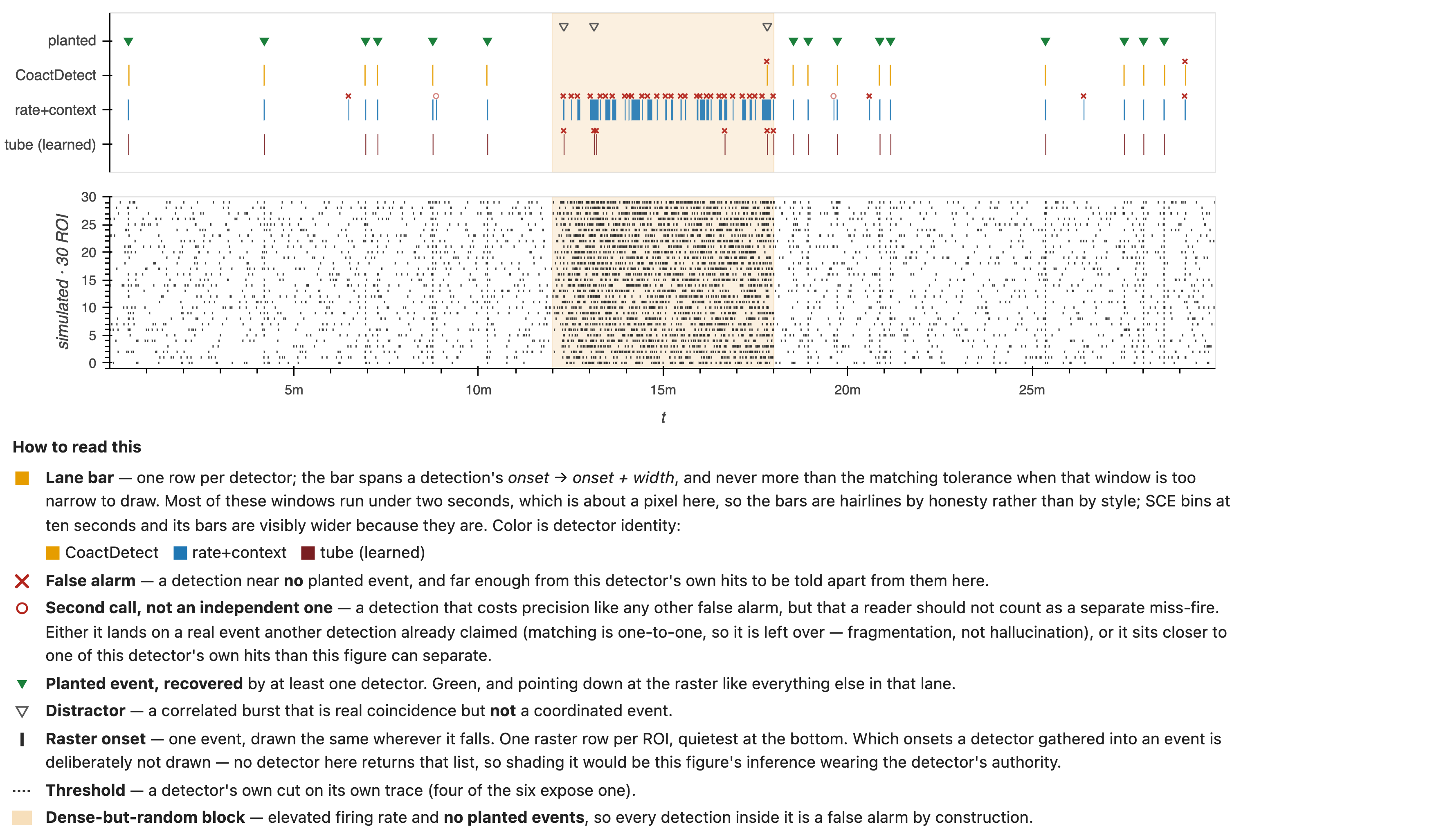
A coordinated event is a moment when many cells in a recording fire together. It is difficult to label them reliably — show two experienced people the same raster and they will not mark the same coordinated events. So the ground truth is planted instead: measure one untreated recording, simulate from those statistics alone, and every event in the training set is there because it was put there.

Eleven hundred parameters. Trains in seconds; scans an hour-long recording in hundredths of one. The learned detector →

Each row above is one ROI — one cell's worth of signal, of the kind pulled out of a 2-photon calcium recording. These rows are simulated and every coordinated event among them was planted, so a miss and a false alarm are drawn rather than inferred.

Detectors flag the moments when many ROIs fire together. There are five in this build — LoCo, SCE, CoactDetect, RateDetect and SPIKE-synch — each asking a different question, and each matched to the MATLAB implementation it was ported from to 1e-9 on committed fixtures. That is a provenance record for the port, and it is not a claim about the published method behind it: matching this lab's MATLAB is not the same as matching the paper. They are calibrated on the same simulation the model is trained on, swept over one declared knob each, and scored by the same rule — which is what makes the comparison a comparison.

There is no single number that settles it, and this page does not pick a winner. On the headline metric the learned models sit level with the best hand-written ones, close enough that their fold ranges overlap. But how often a method fires inside the shaded block — where nothing was planted, so every call is wrong by construction — varies by more than two orders of magnitude across the same set, and the headline metric does not carry it. The learned models span that trade rather than sitting at one end of it: the variant that scores highest is also among the most promiscuous, and a near-identical one gives up almost nothing to fire a fraction as often. Which you would rather have is a question about your recordings, not about the leaderboard.

Why per lab, in full. Between one source of coordination and another the timescales run over many orders of magnitude, along with the sampling rates, the mechanisms, and what even counts as an event. A network trained across all of them comes out mediocre at each. Worse for a working lab: what it learns is the average case, so the preparation that departs from the average is the one it scores as noise — which is the preparation anyone is usually studying.

That synthetic baseline does two jobs at once — it tunes the hand-written detectors and it trains the model, which is what puts them on one benchmark instead of two. Only then is the finished instrument pointed at the whole dataset, treatments included. The treatment is never simulated: simulate it and you have spent the effect you ran the experiment to measure; withhold it and it comes back as a result.

What it cost to get this wrong

Tuning a detector against a synthetic benchmark that does not match reality is not a hypothetical failure here — it happened, and cost two weeks. Settings tuned on a benchmark with events every 14 s collapsed when run on sparse data, because four planted events sat inside every 60 s context window and contaminated the null the detectors depend on. Precision fell from 74% to 10% for one of them.

So the generator carries the things that catch that: a dense-but-random block containing no planted events (a detector fooled by rate lights it up), correlated bursts that are real coincidence but not coordination, and variable event timing, so nothing can be predicted from the clock.

The generator, beside the recording it imitates

Two rasters stacked, each with a lane above it carrying LoCo's calls.
Top, a real recording: most rows nearly empty, a few dense, activity
arriving in bursts. Bottom, the generated imitation: events spread
evenly across every row and all 30 minutes, with the planted events
marked in its lane. — **The match is in the numbers, not in the shape.** The ROI count, the duration, the per-ROI rate, the participation and the jitter are the same above and below. The texture is not: a real field has a few ROIs carrying most of the activity and many carrying almost none, and what activity there is arrives in bursts, while the generator spreads events evenly — across every ROI, and across the whole recording.

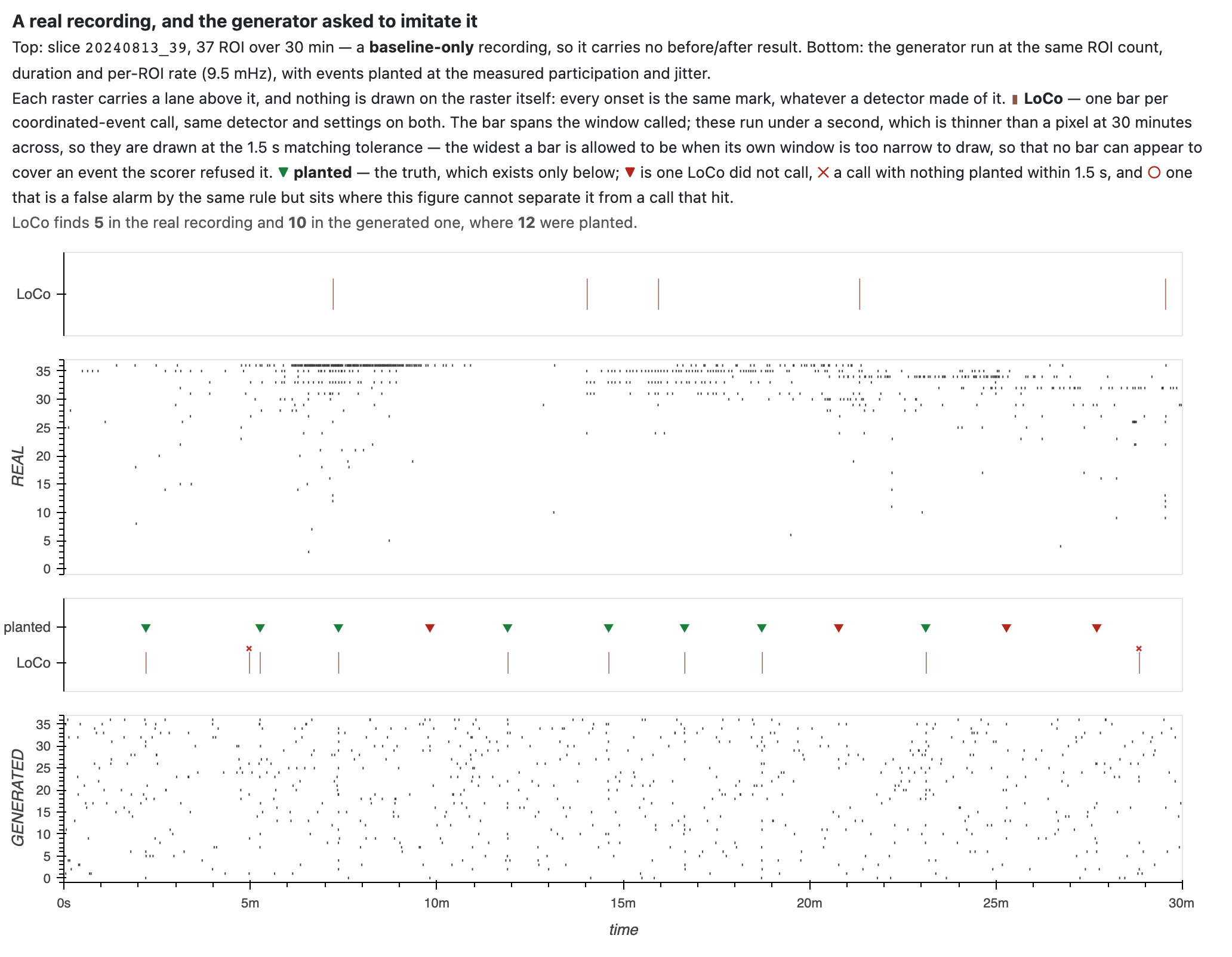
All five work by finding moments that stand out from the rest of the recording, which is what makes the shape of the background more than a cosmetic detail: on the pair above, the same detector at the same settings finds twice as many coordinated events in the imitation as in the original. Matching the rate, the jitter and the participation is necessary and not sufficient. That gap is open work, and it is written down rather than papered over.

One real recording; everything else is synthetic. The top panel above is a real baseline-only slice, published deliberately — it carries no before/after result, so releasing it costs nothing this lab intends to publish. It is a committed figure rather than a live read: the build opens no data store, and generates every other figure here from a seed.

Where this sits, and who else is doing it

Detecting coordinated events is not a new problem, and a page that positions itself against work a reader cannot go and look at is marketing. So: four methods already train networks whose output is a population event with times — DOSED on sleep EEG, cnn-ripple on hippocampal LFP, SEED on sleep spindles and K-complexes, and SpikeNet on clinical EEG, the last of which we have on its bibliographic record alone. None of those four works on calcium imaging, and all four learn from events a human expert labeled. Here the events are planted in a simulation fitted to one lab's own recordings, so the ground truth is exact and the benchmark is rebuilt per lab.

None of that is a first, and it does not need to be. Population-event detection on calcium imaging is already done by non-learned rules — including by the author of the measure SPIKE-synch runs on, who applied it to wide-field calcium imaging (Kreuz et al. 2022, J Neurosci Methods 381:109703). Training on planted rather than expert-marked events is not new either: SpindleNet (2019) used synthetic spindles for the reason argued at the top of this page, and DeepWonder (2023) trains on synthetic recordings outright. We have not found a learned detector emitting population coordinated events with times on calcium imaging — but that is a search that came up empty, not a proof, and fields where planting signals in real background is routine (gravitational-wave astronomy, seismology, high-energy physics) have not been searched at all.

The classical side of the same problem is the coactivity-vs-shuffle rule, and it is already in the figure at the top of this page: binned SCE is that rule itself. Its root is Mao, Hamzei-Sichani, Aronov, Froemke & Yuste (2001), Dynamics of spontaneous activity in neocortical slices, Neuron 32:883–898 — the interval reshuffling that Cossart, Aronov & Yuste (2003) cite as their own reference 12 and apply to UP states in Attractor dynamics of network UP states in the neocortex, Nature 423:283–288. Cite those, not this repo, for the rule. SPIKE-synch is our detector on someone else's measure: the measure is Kreuz, Mulansky & Bozanic (2015), SPIKY: a graphical user interface for monitoring spike train synchrony, J Neurophysiol 113:3432–3445. Where each of the five comes from → carries the rest of the citations, and none of the five is this project's method.

No method from the literature has been run here in its own form.

Open your own recordings

The raster viewer → — point it at a folder of event times and it draws them. It reads the import contract: one CSV per recording with roi and time_sec, which most labs can write from whatever their detector already produces. Your files never leave your computer — the page has no network call in it, and this site is static files with no server to receive anything. Nothing is installed and nothing is uploaded.

No recordings to hand? The same page will invent a folder — event times drawn from the generator described above, written as the contract describes and read back through the same loader, so what you drive is the viewer rather than a demonstration of it. It opens at the measured settings: about six of thirty-three ROIs per coordinated event, a third of a second of spread, and a background whose quiet tail is the fitted one. The guesses those replaced are left on the switches, because the difference is worth seeing. Its treatment windows are labels over identical statistics — simulating an effect would spend the one the experiment exists to measure.

Source: github.com/syncytium2/bugarach · BSD-3-Clause · built from 7208e44